
Abstract: In the last decade, deep learning based generative models have gained more and more attention due to their tremendous progress. Among these models, there are two major families of them that deserve extra attention: Generative Adversarial Networks (GANs) and Variational Autoencoders (VAEs). As a generative model comparable to GANs, VAEs combine the advantages of the Bayesian method and deep learning. It is built on the basis of elegant mathematics, easy to understand and performs outstandingly. Its ability to extract disentangled latent variables also enables it to have a broader meaning than the general generative model. A VAE can be defined as being an autoencoder whose training is regularised to avoid overfitting and ensure that the latent space has good properties that enable the generative process. In this post, VAE will be used to generate digit images based on the MNIST dataset.
Method
In short, as one of state-of-art generative models, a VAE is an autoencoder whose encodings distribution is regularised during the training process to ensure that its latent space has good performance allowing it to generate new data that is not included in the training dataset. It is worth noting that the term “variational” comes from the close relationship between regularization in statistics and variational inference methods. Just like a standard autoencoder, a variational autoencoder is composed of both an encoder and a decoder, as shown in Figure 11, and that is trained to minimize the reconstruction error between the decoded output and the initial data. However, in order to introduce some regularisation of the latent space, the encoding-decoding process is slightly modified by encoding the input as a distribution on the latent space instead of encoding it as a single point. In practice, the encoded distributions are chosen to be normal so that the encoder can be trained to return the mean and the variance matrix that describes these Gaussians. The reason for encoding the input as a distribution with a certain variance instead of a single point is that it can express latent spatial regularization very naturally: the distribution returned by the encoder is forced to be close to the standard normal distribution. 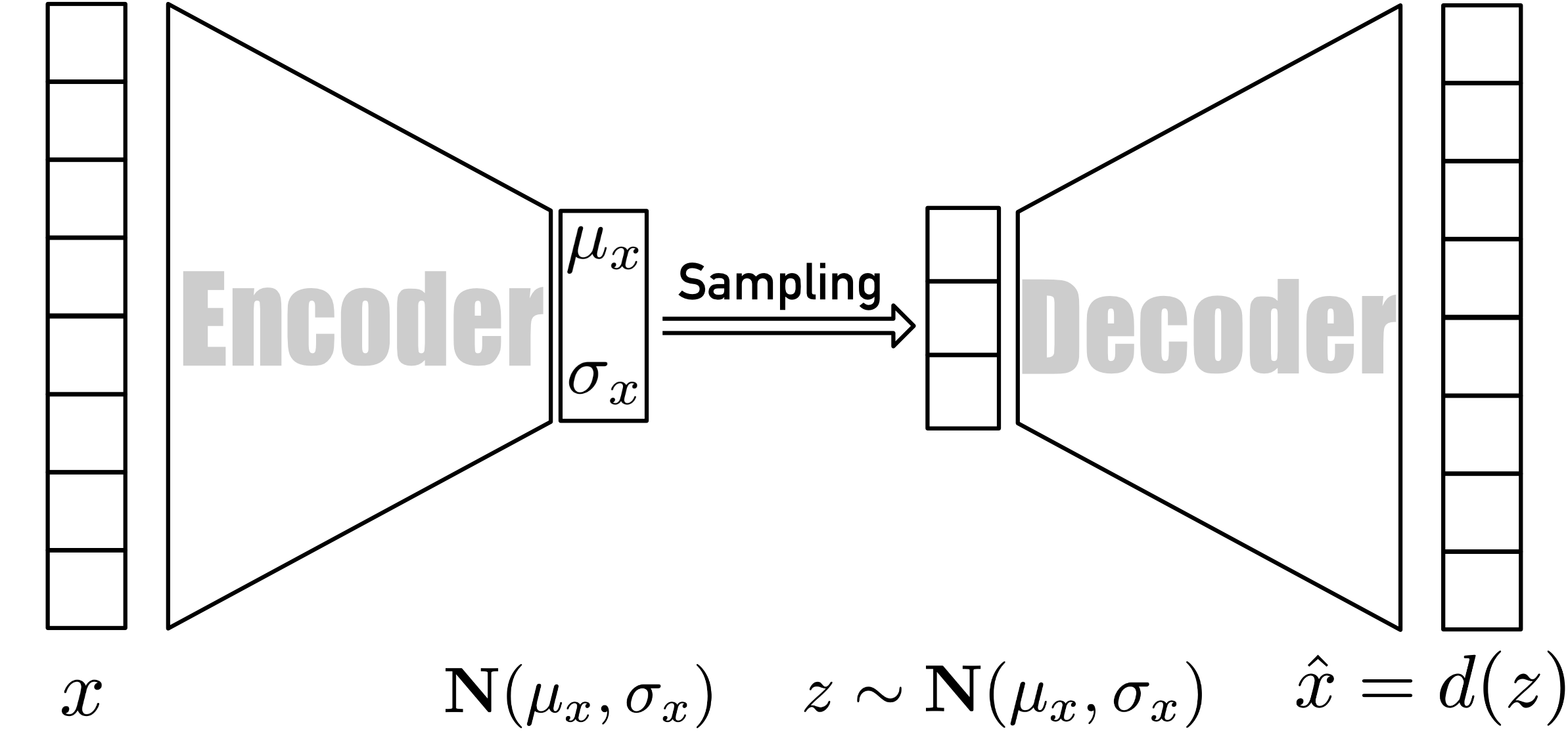 Figure 1. Overview of VAE architecture
Therefore, we can intuitively infer that the loss function of a VAE model consists of two parts: a “reconstruction term” that tends to make the encoding-decoding scheme as good as possible and a “regularisation term” that tends to regularise the organisation of the latent space by making the distributions returned by the encoder close to a standard normal distribution, which can be written as
\[L = ||x-\hat{x}||^2+\mathbb{KL}(\mathbf{N}(\mu_x, \sigma_x),\mathbf{N}(0, 1))\]This function is also called evidence lower bound (ELBO) loss, which will be derived in Theoretical Part. As you can see, the regularisation term is expressed as the Kulback-Leibler divergence (KL) between the returned distribution and normal distribution. We can notice that the KL divergence between two Gaussian distributions has a closed form that can be directly expressed in terms of the means and the covariance matrices of the the two distributions. In this report, the mean-squared error (MSE) is applied to calculate the reconstruction loss, which is defined as
\[\text{MSE} = \frac{1}{n}\sum_{i=1}^n||x-\hat{x}||^2\]where $n$ is the number of training data, and
\[\text{KL Loss} = \sum_{i=1}^n(1+\log(\sigma_i^2)-\mu_i^2-\sigma_i^2)\]is applied for calculating the KL divergence.
Next, we will discuss the encoder and the decoder. The output of an encoder is a compressed representation which is called latent variable and the decoder takes it as input and tries to recreate the original input data. In practice, these two parts can be implemented using two neural networks. In this report, two convolutional neural networks (CNN) are used with details shown in Table 1 and 2. It is worth noting that the reason why the dimension of the fully connected layer of encoder used here is 40 is that half of it is used as mean, and the other half is used as variance so that the length of latent space is 20. Moreover, transposed convolution layers are applied in decoder to up-sample the latent variables.
| Layer | Input Size | Filter Size | Stride | Output Size |
|---|---|---|---|---|
| conv1 | $28^2\times1$ | $3^2\times32$ | 2 | $14^2\times32$ |
| conv2 | $14^2\times32$ | $3^2\times64$ | 2 | $7^2\times64$ |
| fc | $7^2\times64$ | - | - | $40$ |
| Layer | Input Size | Filter Size | Stride | Output Size |
|---|---|---|---|---|
| tconv1 | $1^2\times20$ | $7^2\times64$ | 7 | $7^2\times64$ |
| tconv2 | $7^2\times64$ | $3^2\times64$ | 2 | $14^2\times64$ |
| tconv3 | $14^2\times64$ | $3^2\times32$ | 2 | $28^2\times32$ |
| tconv4 | $28^2\times1$ | $3^2\times1$ | 2 | $28^2\times1$ |
As we discussed before, before minimizing the loss, we need to generate sampled data, which includes the mean and the variance vectors to create the final encoding to be passed to the decoder network. However, we need to use back-propagation later to train our network later so that we cannot do sampling in a random manner. In this case, the trick of reparameterization can be adopted to substitute for random sampling. As shown in Figure 2, it is an example of our model with the length of latent variable equal to three and you can see that the the latent space
\[z_i=\mu_i+\exp{(\sigma_i)}\times e_i\]where $e_i\sim\mathbf{N}(0,1)$. The general idea is that sampling from $\mathbf{N}(\mu_i,\sigma^2)$ is same with sampling from $\mu_i+\exp{(\sigma_i)}\times e_i$.
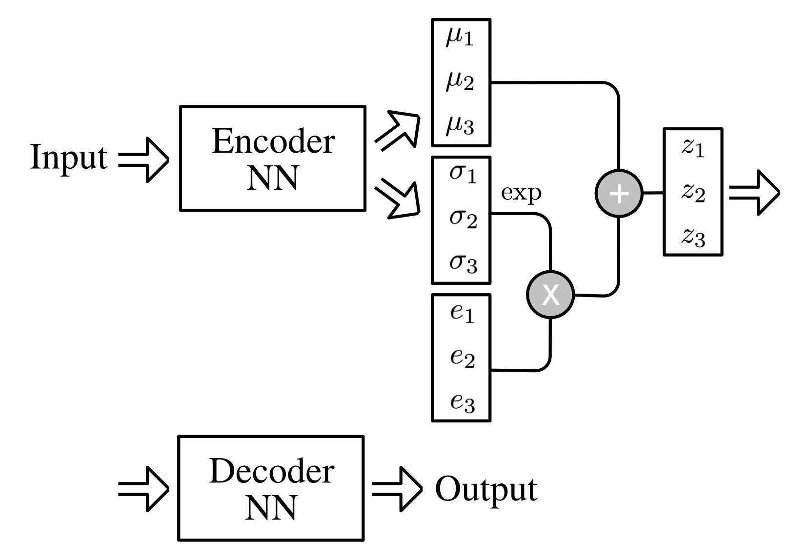 Figure 2. VAE with reparameterization
Experiment and Evaluation
Now that we have defined everything we need, it is time to get it trained. The training parameters are shown in Table 3 and momentum is used in this report. The training progress plot is shown in Figure 3, the loss stays at around $18.5\%$ after 50 epochs of training.
| Epochs | Learning Rate | Gradient Decay Factor |
|---|---|---|
| 50 | 0.001 | 0.9 |
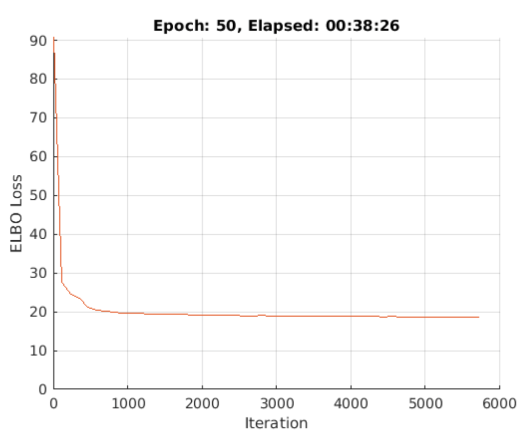 Figure 3.Training progress plot of VAE</center>_
Now, let’s evaluate our trained VAE. First of all, randomly select ten images with labels of 0-9 from the test set and pass them through the encoder, and then use the decoder to reconstruct the images using the obtained representation. Shown in Figure 4, in most cases, after the encoding-decoding process, the reconstruction result is quite good, but for some input images whose writing is not in standard style, errors will occur. In addition, by observing these reconstructed images, we can find that the images generated by VAE are usually blurry.
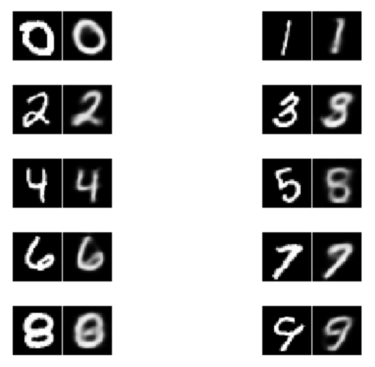 Figure 4. Reconstruction images of each digit
Now, let’s generate some new images. Randomly generate a number of encodings from normal distribution with the length same with the latent space and pass them through the decoder to reconstruct the images, the results are shown in Figure 5. In addition to the phenomenon mentioned before that the generated image will get blurred, it is not difficult to see that some generated images are meaningless, such as the image in the fourth row and fifth column, since it is hard to determine whether it’s a 4 or 9.
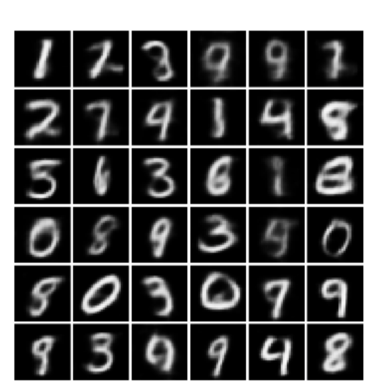 Figure 5. Randomly generated samples of digits
In fact, compared with some models I tried before, the test result of the current model is one of the most satisfactory ones. Previously, I tried to add pooling layers and use shorter hidden variables, but the results were very bad. Some examples are shown in Figure 6. Apparently, using pooling layer to down-sample the image is not a good choice here for encoder and the length of latent variable should not be too short.
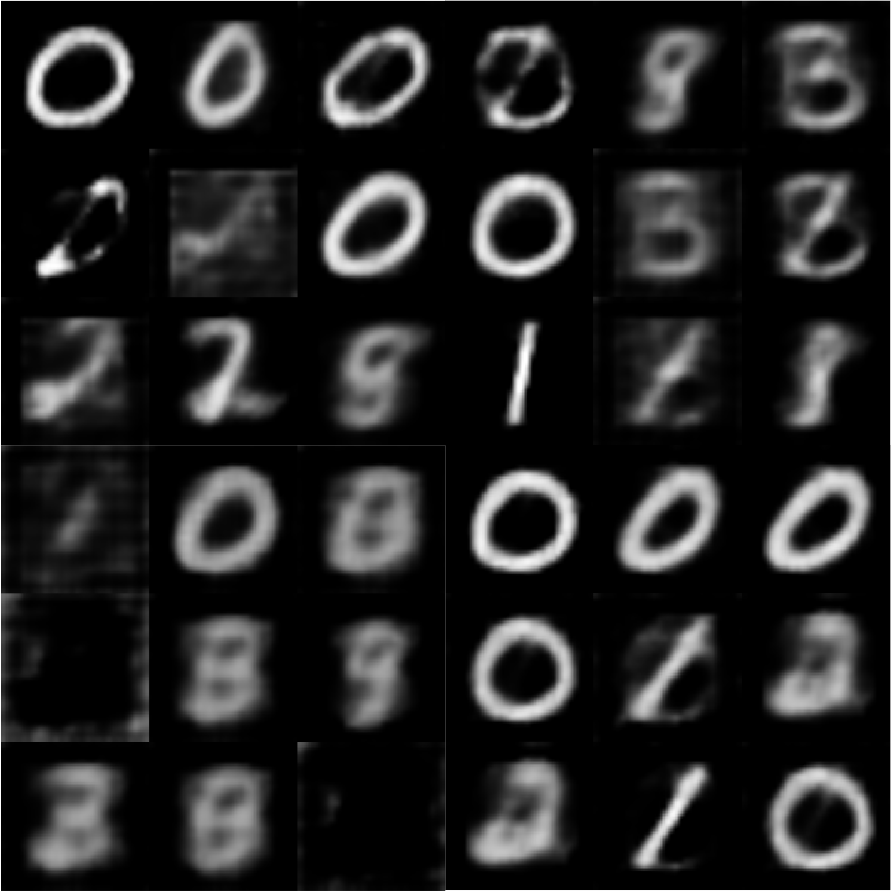 Figure 6. Image generated by the model in case of failure
In the experiment, the classifier network architecture is shown in Table 4 below and the softmax function is applied on the final output of the network to obtain the classification result. After training on the entire training set of MNIST, the accuracy for testing on the test set can reach 99.21%.
| Layer | Input Size | Filter Size | Stride | Output Size |
|---|---|---|---|---|
| conv1 | $28^2\times1$ | $3^2\times8$ | 1 | $28^2\times8$ |
| BN | $28^2\times8$ | - | - | $28^2\times8$ |
| mp1 | $28^2\times8$ | $2^2$ | 2 | $14^2\times8$ |
| conv2 | $14^2\times8$ | $3^2\times16$ | 1 | $14^2\times16$ |
| BN | $14^2\times16$ | - | - | $14^2\times16$ |
| mp2 | $14^2\times16$ | $2^2$ | 2 | $7^2\times16$ |
| conv3 | $7^2\times16$ | $3^2\times32$ | 1 | $7^2\times32$ |
| BN | $7^2\times32$ | - | - | $7^2\times32$ |
| fc | $7^2\times32$ | - | - | $10$ |
Following the instruction, using half of the MNIST training set to train the VAE model defined in last section and use it to generate new images. The process of generating new images is as follows: re-input the training set used for training VAE to the encoder and get its encoding, add some Gaussian Noise to a portion of the encoding and then pass it through the decoder to regenerate new images. The generated image can refer to Figure 5, whose result is generally consistent. Use a certain proportion of unused training data in MNIST together with the same amount of newly generated data to train the classifier defined in Table 4, and use the test set in MNIST to test the trained classifier. The accuracy of the tests is shown in Table 5. As you can see, when the amount of training data increases, the accuracy of the test also increases. This is not difficult to explain, but what is interesting is that these test results are not as good as the classifier trained with the entire MNIST training set. I think the reason may be because the MNIST dataset is so easy that adding some interference does not improve the generalization ability of the classifier. However, I think for some more difficult datasets, doing this will reduce the overfitting and improve the classification ability.
| Percentage (%) | 20 | 50 | 100 |
|---|---|---|---|
| Accuracy (%) | 97.50 | 98.34 | 98.70 |