Abstract: The project aims to provide a demo animal detection model with the long-term goal of developing a phone application. Two different state-of-art algorithms are tested out, one is YOLOv5 and another is Faster R-CNN. These two represents two different families of detection methods, one is one-stage while another is two-stage. YOLO is an end-to-end target detection framework that transforms target detection into regression problems while R-CNN is a target detection framework combining region proposal and CNN classification. We compare the two algorithms in accuracy and speed and found that YOLOv5 performs better in both aspects. At the end of this report, there will be some discussion about the results and methods to further expand the model in the future.
Introduction
As one of the most potent public education organisations, Universeum is a public arena for lifelong learning where children and adults explore the world through science and technology. This project is for building an animal detection model based on deep learning methods. Doing so can help Universeum further develop related mobile applications in the future, thereby making it easier to convey knowledge and information to tourists. In this project, we collected and annotated our own dataset, which contains 19 classes of animals. The method of data augmentation is performed to generalize new images and introduce them to the networks. Then, the transfer learning method would be applied and feed the dataset to two state-of-art pre-trained networks, YOLOv5 and Faster R-CNN.
Related Work
Object detection, as of one the most fundamental and challenging problems in computer vision, has received significant attention in recent years. It is an important computer vision task that detects visual objects of certain classes in digital images. In the deep learning era, object detection can be categorized into two groups1: “two-stage detection” and “one-stage detection”, where the former frames the detection as a “coarse-to-fine” process while the latter frames it as to “complete in one step”. In this project, two different detectors from each category are tried out, YOLOv5 and Faster R-CNN.
You Only Look Once (YOLO)
YOLO was primely proposed by R.Joseph et al. in 2015, which is the very first one-stage detector2. Compared to the approach taken by object detection algorithms before YOLO, YOLO proposes using an end-to-end neural network that makes predictions of bounding boxes and class probabilities all at once. YOLO provided a super fast and accurate object detection algorithm that revolutionized computer vision research related to object detection. It applies a single neural network to the full image, which divides the image into regions and predicts bounding boxes and probabilities for each region simultaneously. R. Joseph has made a series of improvements on the first version and proposed version 2 and 3 editions34 but then he left the community last year, so YOLOv4 and later versions are not his official work. However, the legacy continues through new researchers. In this project, we decided to use the latest model of the YOLO family, version 5, which is an open-source project that consists of a family of object detection models and detection methods based on the YOLO model pre-trained on the COCO dataset.
How YOLO works
The YOLO algorithm works by dividing the image into $N$ grids, each having an equal dimensional region of $S \times S$. Each of these $N$ grids is responsible for the detection and localization of the object it contains. Correspondingly, these grids predict bounding boxes relative to their cell coordinates, along with the object label and probability of the object being present in the cell. This process greatly lowers the computation as both detection and recognition are handled by cells from the image. However, it brings forth a lot of duplicate predictions due to multiple cells predicting the same object with different bounding box predictions. YOLO makes use of Non-Maximal Suppression (NMS) to deal with this issue. In NMS, YOLO suppresses all bounding boxes that have lower probability scores. YOLO achieves this by first looking at the probability scores associated with each decision and taking the largest one. Following this, it suppresses the bounding boxes having the largest IOU with the current high probability bounding box. This step is repeated till the final bounding boxes are obtained.
There are two parts to the loss function, bounding box regression loss and classification loss. In terms of b-box regression loss, IOU loss was used in the past. The latest models use deformations based on this loss, such as CIOU Loss and DIOU Loss.
YOLO Architecture
YOLO is designed to create features from input images and feed them through a prediction system to draw boxes around objects and predict their classes. Since YOLOv3, the YOLO network consists of three main pieces.
- Backbone: A convolutional neural network that aggregates and forms image features at different granularities.
- Neck: A series of layers to mix and combine image features to pass them forward to prediction.
- Head: Consumes features from the neck and takes box and class prediction steps.
There are abundant approaches that can be used to combine different architectures at each component listed above. The contributions of YOLOv4 and YOLOv5 first integrate breakthroughs in other fields of computer vision and incorporate them into the original YOLO structure to improve performance.
Faster R-CNN
Faster R-CNN is a member of R-CNN family. R-CNN is published by R. Girsh in 20135. Then some improvements have been made by the author himself, which is Fast R-CNN, published in early 20156. And finally is the model published in the same year, Faster R-CNN7. Figure 1 is the whole structure of Faster R-CNN and the theory will be elaborated below.
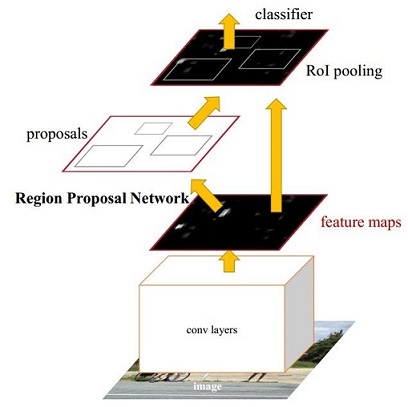 Figure 1. Structure of Faster R-CNN7
Covolutional Layers
As a CNN network target detection method, Faster R-CNN uses basic Covolutional layers like VGG16 or ResNet50 to extract image feature maps. These layers is the cov layers in Figure 1, which is also called base network because the whole structure is built based on it.
The obvious advantage of ResNet over VGG is that it is bigger, hence it has more capacity to actually learn what is needed8.
The feature maps are shared for the subsequent RPN layer and fully connected layer. The VGG16 and ResNet50 are always pretrained to reduce the difficulty in training.
Region Proposal Networks
Classical detection methods are very time-consuming to generate detection frames. For example, sliding windows, which we have learned in class, really needs to iterate so many times; or R-CNN uses SS (Selective Search) method to generate anchor box5. Faster RCNN abandons the traditional sliding window and SS method and directly uses Region Proposal Networks (RPN) to generate the anchor box. This is also a huge advantage of Faster R-CNN, which can greatly improve the generation speed of the detection frame.
Before continue talking about RPN, we want to discuss the anchor box first, which is inherited from R-CNN. Traverse the feature maps calculated by Conv layers, and equip each point with these 9 prior anchors given as hyper parameters as the initial detection frame.
The RPN does two different type of predictions: the binary classification and the bounding box regression adjustment. The loss of fist prediction is cross entropy loss and the second is L1 loss:
\[Loss = \sum^{N}_{i}{|t_*^i - W_*^T\cdot \phi(A^i)|} + \lambda ||W_*||.\]Here $t_*^i$ is the target box and $W_*^T\cdot \phi$ is the linear map of anchor box.It should be clear that only when the distance between two boxes is short enough, can the map be viewed as linear.
There are some many anchors, so we introduced Non-Maximum Suppression (NMS). NMS discards those proposals that have a score larger than some predefined threshold with a proposal that has a higher score.
RoI Pooling
The Region of Interest (RoI) Pooling layer is responsible for collecting proposals, calculating proposal feature maps, and sending them to the subsequent network.
For traditional CNN (such as AlexNet and VGG), when the network is trained, the input image size must be a fixed value. Faster R-CNN tries to solve this problem by reusing the existing conv network. This is done by extracting fixed-sized feature maps for each proposal using region of interest pooling. Fixed size feature maps are needed for the R-CNN in order to classify them into a fixed number of classes.
Classification
The probability vector is obtained by fully connected layer and softmax. Bounding box regression is used to obtain each proposal’s position offset in order to return to a more accurate target detection frame.
Methodology
In this section, we will see how we conduct our project in detail.
Dataset
At the very soul of training deep learning networks is the training dataset. The first step of any object detection model is collecting images data and performing annotation. For this project, we went to the museum in person and manually collected 764 images of real scenes. Training datasets are images collected as samples and annotated for training deep neural networks. For object detection, there are many formats for preparing and annotating your dataset for training. The most popular formats for annotating an object detection datasets are Pascal VOC, Micosoft COCO, and YOLO format. Since we intend to use transfer learning, YOLO and Faster R-CNN require different formats of annotations, so two different annotation formats have been prepared, VOC and YOLO formats.
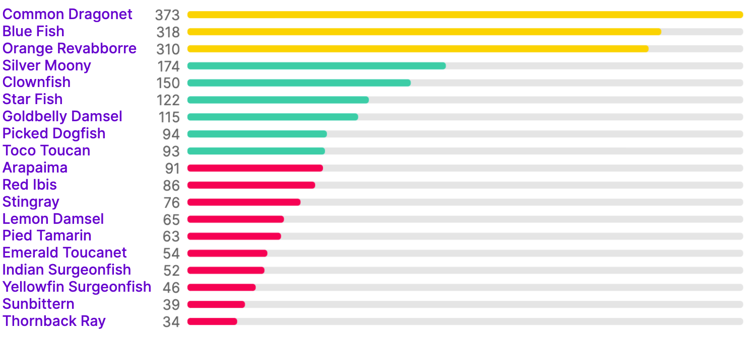 Figure 2. Class balance of the collected and annotated dataset
There are in total 19 classes of animals appeare in our collected datset. However, we can see from the Figure 2 that our data set is unbalanced. Some animals have been labeled more than 300 while some have fewer than 50. This factor needs to be considered in the analysis of the final result. All images are then resized into 416 by 416 and the entired dataset is randomly divided into training, validation, and test set according to the ratio of 7:2:1.
Image augmentation is a method to increase the generalizability of your model’s performance by increasing the diversity of learning examples for your model. Specific methods include rotation, flipping, and brightness adjustment. We performed this process on the training set and expanded it by a factor of two.
Transfer Learning
Since we only have a small dataset, in order to obtain a good model in time, the transfer learning method is adopted. We separately train on pre-trained YOLOv5 model and Faster RCNN model.
YOLO
YOLOv5 is an open-source project that consists of a family of object detection models. Since the model will be potentially deployed on mobile phones, smaller models are preferred. Therefore, the smallest YOLOv5 architecture, YOLOv5s, is then selected to be trained on. The pre-trained models are available in their github page. 100 epochs of training are preformed.
Faster RCNN
Pretrained models of Faster R-CNN are downloaded online in this page and here. Compared to the original paper, we set smaller prior anchor box to detect small objects. We use two base models, VGG16 and ResNet50 to fulfill the task. Training epoch is 50, of which 30 is trained while base model is frozen while 20 unfrozen. Learning rate is $10^{-4}$ for frozen part and $10^{-5}$ for unfrozen with decaying.
Results
We calculate the mAP of two algorithms and results are shown in Table 1. Both of these detectors perform well for detecting large animals, but for small animals that look very similar (especially some fish), both models perform relatively poorly but each has its own merits. Note that this result does not truly reflect the true ability of these two detectors, because the dataset is very limited (the test set has only 76 images). However, this result can also be used as a reference to test the performance of these two models on this specific task.
| Method | YOLOv5 | Faster R-CNN |
|---|---|---|
| all | 0.82 | 0.74 |
| Arapaima | 0.64 | 0.81 |
| Orange Revabborre | 0.97 | 0.70 |
| Stingray | 0.96 | 0.73 |
| Toco Toucan | 0.76 | 0.90 |
| Emerald Toucanet | 0.99 | 1.00 |
| Pied Tamarin | 0.46 | 0.40 |
| Sunbittern | 1.00 | 1.00 |
| Goldbelly Damsel | 0.78 | 0.31 |
| Lemon Damsel | 0.88 | 0.66 |
| Red Ibis | 0.88 | 1.00 |
| Thornback Ray | 0.64 | 0.95 |
| Picked dogfish | 0.91 | 0.71 |
| Clownfish | 0.89 | 0.64 |
| Common dragonet | 0.92 | 0.74 |
| Starfish | 0.70 | 0.66 |
| Indian Surgeonfish | 0.55 | 0.79 |
| Yellowfin surgeonfish | 1.00 | 1.00 |
| Silver Moony | 0.76 | 0.12 |
| Blue Fish | 0.96 | 0.81 |
Besides, we measure the average fps of two algorithms when predicting videos in Table 2. The whole experiment is implemented on a GeForce RTX 2060 SUPER.
| Method | YOLOv5 | Faster R-CNN |
|---|---|---|
| fps | 200.00 | 8.37 |
Conclusions
In the above table, we just show the best result of Faster R-CNN and now the comparison between VGG16 and ResNet50 is shown in Table 3.
| Faster R-CNN VGG | Faster R-CNN ResNet | |
|---|---|---|
| mAP | 0.74 | 0.72 |
| fps | 8.37 | 3.93 |
The mAP of VGG is slightly better than ResNet while fps is two times better surprisingly. We think it is because our task is relatively simple. The main difference between VGG and ResNet is that ResNet has bigger network, which means it will definitely run slower, but for a simple task, the advantage of extracting more information is not shown.
According to common sense, one-stage algorithm is faster while two-stage algorithm is more accurate. There is no surprise to see YOLOv5 is greatly quicker while a bit more correct since YOLO has fixed its disadvantage in detecting small objects since YOLOv3 and nowadays YOLOv5 also draw lessons from R-CNN. But it is still strange to observe such a bad performance in small objects (Sliver Moony) with Faster R-CNN. So we check it thoroughly and find the problem, that is, the only two pictures of Silver Moony in the test set is so blurry that even a human can not recognize it easily. We tried another picture borrowed from another group and find it work fine. Since it is quite time-consuming to shuffle the train, validation as well as test set and retrain them, we just clarify the fact here.
Since the long-term goal of this project is to develop an animal recognition application for Universeum, we also need to consider the scalability of the model. In theory, this should be very easy. Take YOLOv5 as an example, just change the output dimension of the output layer to the required number, and perform a few rounds of training on the expanded dataset (not verified), and you should be able to get a well performed expanded model. Of course, in order to ensure that the model performs good, the quality and data content of the dataset should be better.
Reference
Z. Zou, Z. Shi, Y. Guo, and J. Ye, “Object detection in 20 years: A survey,” arXiv preprint arXiv:1905.05055, 2019. ↩
J. Redmon, S. Divvala, R. Girshick, and A. Farhadi, “You only look once: Unified, real-time object detection,” in Proceedings of the IEEE conference on computer vision and pattern recognition, 2016, pp. 779–788. ↩
J. Redmon and A. Farhadi, “YOLO9000: better, faster, stronger,” in Proceedings of the IEEE conference on computer vision and pattern recognition, 2017, pp. 7263–7271. ↩
J. Redmon and A. Farhadi, “Yolov3: An incremental improvement,” arXiv preprint arXiv:1804.02767, 2018. ↩
R. Girshick, J. Donahue, T. Darrell, and J. Malik, “Rich feature hierarchies for accurate object detection and semantic segmentation,” arXiv e-prints, p. earXiv:1311.2524, Nov. 2013. ↩ ↩2
R. Girshick, “Fast R-CNN,” arXiv e-prints, p. earXiv:1504.08083, Apr. 2015. ↩
S. Ren, K. He, R. Girshick, and J. Sun, “Faster R-CNN: Towards Real-Time Object Detection with Region Proposal Networks,” arXiv e-prints, p. earXiv:1506.01497, Jun. 2015. ↩ ↩2
K. He, X. Zhang, S. Ren, and J. Sun, “Deep Residual Learning for Image Recognition,” arXiv e-prints, p. earXiv:1512.03385, Dec. 2015. ↩